

Журнал высшей нервной деятельности им. И.П. Павлова, 2023, T. 73, № 6, стр. 857-872
WEEGIT – software for visualization and annotation of the electrophysiological activity registration data
D. S. Suchkov a, *, V. V. Shumkova b, V. R. Sitdikova b, V. M. Silaeva b, A. E. Logashkin b, A. R. Mamleev b, M. G. Minlebaev a, b
a INSERM UMR1249, INMED, Aix-Marseille University
Marseille, France
b Kazan Federal University
Kazan, Russia
* E-mail: suchkov.dmitriy.ksu@gmail.com
Поступила в редакцию 11.08.2023
После доработки 31.08.2023
Принята к публикации 31.08.2023
- EDN: IKLQWI
- DOI: 10.31857/S0044467723060102
Аннотация
Wizard for EEG Information Tabling – “WEEGIT” is a software designed for visualization and annotation of the long-lasting records of activity. Long-lasting records of raw data are used in various areas of life sciences and well represented in neuroscience. In spite of development of other techniques and approaches the electrophysiological activity registration remains the “golden standard” in neurobiological research. Therefore, we developed and verified “WEEGIT” as a powerful and convenient tool for electrophysiological recordings’ description. We combined the most important features presented in other commercial and noncommercial software in the “WEEGIT”. Presented software can operate with widely used formats of records. ”WEEGIT” allows adaptive visualizing of up to 512 channels of record in different timescale without loss of efficiency and consumption of large machine resources. Visualizing also includes optional built-in temporal-spatial analysis (density of current sources or the density of action potentials) displayed as a background image. Integration of a set of optional filtering and signal transforming procedures allows improving record visualization. “WEEGIT” has a convenient graphical user interface with opportunity of simultaneous time browsing and annotating of the records in one workspace. Annotation can be done by simple text information typing as well as an interactive placing of specialized labels and objects. Software also allows saving data in the resampled format, both for the whole record and for user-defined events. In conclusion, “WEEGIT” provides a great set of benefits for the convenient workflow for beginners and specialists in the electrophysiological area of research, including preparation of the data for further specialized analysis.
1. INTRODUCTION
Despite of wide usage of the optogenetic approaches, electrophysiological recordings (invasive and non-invasive extra-/intracellular recordings in vitro and in vivo) are still the main tool for the neurophysiological research both in science and medicine. Recently, developing technologies have led to significant increase in resolution of electrophysiological data both in space and in time domain. Altogether, with simultaneous recordings of the telemetric information, that provided a huge set of data for research and diagnosis. A large variety of modern analytical packages showed exciting opportunities for deep analysis of the electrophysiological recordings (Hazan, 2006; Tadel, 2011; Patel, 2017; Siegle, 2017; Nasiotis, 2019). However, during experiment or diagnostics, the first overview of the data doesn’t require all analytical power of the mentioned software. Moreover, verification of the observing patterns of activity very often can be done only visually for the first time. Thus, for the first pre-analysis stage, the operator should be able to annotate recorded electrophysiological information to prepare it for further specialized analysis. This important part of the scientific and diagnostic workflow is a first stage of education of the beginners like postgraduate student or intern. Therefore, complexity of the software architecture and graphical user interface can be a critical point for rapid engagement of them. At the same time, effective interaction between experimenters and analysts was always a cornerstone of scientific workflow. That means, as more documented and representative information was provided by experimenter, as more qualitative will be analysis, and opposite. Therefore, for the first pre-analysis stage software should provide opportunities for easy visualization, annotating, collecting and saving of important episodes of activity in both manual and automatic way. A clear preparation process will simplify interaction in discussion between experimenters and analysts, and provide high efficiency of workflow. Besides that, low skill in programming or neurophysiology area will be leveled by multiple choice of activity detection. Thus, efficient engine for fast visualization and annotation of the electrophysiological recordings are the main keys of the pre-analysis stage. However, representation of large volumes of data also highly sensitive to the hardware, requiring essential machine resources. Obvious solution for downsampling in time and space domain will reduce the quality of the observed patterns and can critically bias conclusions about activity. Therefore, for the effective usage of machine resources, software should avoid uploading the full set of data, while recognition of patterns shouldn’t be affected.
Following the concept described above, we designed a powerful and convenient desk tool for visualization and annotating of the electrophysiological activity registration data. Here, we present WEEGIT software, that combines a fast and efficient visual component with extended text editor opportunity. A simple and intuitive graphical user interface allows the operator to add and edit information about general features of the record as well, as a specific event properties. Software engine provides control of the spatio-temporal resolution of the record with resource-efficient visualization. Altogether, that allows the user to do fast and efficient browsing and annotating of the electrophysiological recordings.
2. WEEGIT GRAPHICAL USER INTERFACE
WEEGIT graphical user interface contains panels for displaying and marking data, dropdown menu tabs and toolbar panel. Some available menu actions are duplicated with buttons or editing opportunity on the panels. The name of the record and status of the applied filter and transform have no unique panel and are placed in the top left part of the graphical user interface.
2.1. Panels
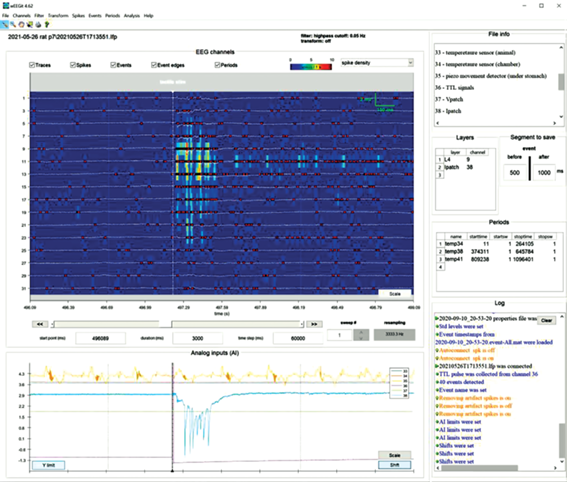
Panels functions can be classified in three groups: 1) graphical representation of the data; 2) editable information about current recording and 3) log of the user actions (Fig. 1).
Fig. 1.
WEEGIT interface view 1, using spike density as background. The main panel (EEG channels) displays amplifier channels extracted from the electrophysiological record. The additional panel (Analog inputs (AI)) displays data from other sensors (e.g., telemetry sensors) synchronized with electrophysiological data. General information panel (File info) is intended for downloading (in *.txt format) and/or creating and editing text information about the current record. The panel of morphological labels (Layers) is used for marking the correspondence of channels to morphological structures. The segment saving panel (Segment to save) contains editable time values defining intervals before and after each event (in milliseconds) that will be used to save data segments around the event timestamp. The period information panel (Periods) is used to enter/edit time period information if the user needs to mark the time period during which the experiment conditions were changed/intact. The action overview panel (Log) displays non-editable information about ongoing user actions. Рис. 1. Вид 1 интерфейса WEEGIT, в качестве фона используется плотность потенциалов действия. На основной панели (EEG channels) отображаются данные регистрации электрофизиологической записи для каждого канала усилителя. На дополнительной панели (Analog inputs (AI)) отображаются данные с других датчиков (например, с телеметрических сенсоров), синхронизированные с электрофизиологическими данными. Панель общей информации (File info) предназначена для загрузки (в формате *.txt) и/или создания и редактирования текстовой информации о текущей записи. Панель морфологических меток (Layers) предназначена для обозначения соответствия каналов морфологическим структурам. Панель сохранения сегментов (Segment to save) содержит редактируемые значения времени, определяющие интервалы до и после события (в миллисекундах), которые будут использоваться для сохранения сегментов данных вокруг временной метки каждого события. Панель информации о периодах (Periods) используется, если необходимо, для ввода/редактирования информации о периоде времени, в течение которого изменялись/сохранялись условия эксперимента. Панель обзора действий (Log) отображает нередактируемую информацию о действиях пользователя.
EEG channels. The main panel “EEG channels” displays amplifier channels extracted from the electrophysiological record. “EEG channels” panel is consisted of 1) attributes control space (upper position); 2) main axes with record data (middle position) and 3) navigation control space with time and sweep control elements (bottom position). During session saving, all parameters of the elements on the “EEG channels” panel are saved in an additional 〈filename〉. WEEGITweegit.mat file. During connecting to the 〈filename〉.lfp, an additional file 〈filename〉. WEEGITweegit.mat will be automatically uploaded (if it exists) and state of the elements on the “EEG channels” panel from the last session will be restored (see “File” → “Save session settings” in “Menu” section and “Session” in “Methodology” section).
Attributes control space. “Attributes control space” is intended for user regulation of graphical elements’ presence in the “Main axes”. The left part of “attributes control space” includes ticks to visualize/hide on the main panel the following attributes: “traces”, “spikes”, “events”, “event edges” and “periods”. Right part of attributes control space presented by reserved space for the background color-code horizontal bar (on the left) and background selection popup menu (on the right). Background selection popup menu offers three modes: 1) “CSD” (current source density); 2) “spike density” and 3) “nothing”. “Spike density” mode selection starts evaluation of the average spike’s number in the adaptive sliding window (Fig. 1). “CSD” mode selection starts evaluation of the current source density distribution, base on the second spatial derivative (Buzsaki, 2012) between each signal presented in main axes (fig. 2). That, in a certain manner, provided information about spike rate at the moment. The size of sliding time window is adaptively changing according to the signal window time range. That provide remarkable representation of the spike density in a different time scales, however, spike rate in this case may be biased according to the scale. “Nothing” mode remove background from the “Main axes” (Fig. 3).
Fig. 2.
WEEGIT interface view 2, using current source density (CSD) as a background. The upper drop-down menu contains sets of actions for: converting/loading/saving data (File); changing display settings (Channels); filtering data (Filter); transforming data (Transform); detecting action potentials (Spikes); detecting/labeling/saving events (Events); setting/editing time periods (Periods); initial analysis of events (Analysis); studying the basic functionality of the program (Help). Рис. 2. Вид 2 интерфейса WEEGIT, в качестве фона используется плотность источников тока (ПИТ). Верхнее выпадающее меню содержит наборы действий для: конвертации/загрузки/сохранения данных (File); изменения настроек отображения (Channels); фильтрации данных (Filter); преобразования данных (Transform); обнаружения потенциалов действия (Spikes); обнаружения/маркировки/сохранения событий (Events); установки/редактирования временных периодов (Periods); первичного анализа событий (Analysis); изучения основных функциональных возможностей программы (Help).
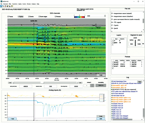
Fig. 3.
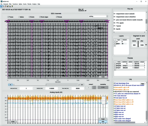
WEEGIT interface view 3, no background. Example of ∼30 min of record. Рис. 3. Вид 3 интерфейса WEEGIT, без фона. Пример отображения ∼30 мин записи.
Main axes. “Main axes” contains graphical representation of the objects “traces”, “spikes”, “events”, “event edges”, “periods” and background image. “Traces” are record data, organized vertically, where each row contain signal from one single electrode. Represented as vertical solid black lines (if background is “nothing” or “CSD”) or as vertical solid white lines (if background is “spike density”). “Spikes” are action potentials, high-frequency events with duration from 1 to 2 ms, extracted from each signal in user-defined way. This type of graphical objects is specific for recordings with high-impedance electrodes and optional for other types of electrophysiological recordings. Timestamps for spikes represented as red (default) squares horizontally aligned to the source channel position. In future release, color will represent affiliation to cluster. “Events” are customized events’ times, defined and prepared by user. Represented as vertical dash-dotted black line (if background is “nothing” or “CSD”) or as vertical dash-dotted white lines (if background is “spike density”) with triangle on the end. Each event has a unique name, displayed by text with the same color as the line. If event set as “bad” the color of line and text becomes red for any background. ”Event edges” are boundaries for the segment around each event, which times are defined in the “Segment to save” panel. Represented as vertical dotted black line (if background is “nothing” or “CSD”) or as vertical dotted white lines (if background is “spike density”). “Periods” – boundaries for the user defined time periods of interest. Represented as vertical solid magenta line. Period’s left boundary name displayed as magenta dual-line text and consist of user-defined name (top) and “start” string (bottom). Period’s right boundary name displayed as magenta dual-line text and consist of user-defined name (top) and “stop” string (bottom). The y-axis of the “Main axes” contains numbers of the record channels.
The background image is defined by the user through the background selection popup menu. Only the current configuration of channels will be used for the background build, if channels are hidden or sorted by user management (see “Channels” → “Configure EEG” in “Menu” section). The resulted background image is displayed as a background image in jet color code. The background color-code horizontal bar shows the color correspondence between values and colors. The “Scale” push button placed in the bottom left corner of the main axes. Pushing this button calls the user dialog with three fields: “Scale factor”, “Scale units” and “Background scale”. The value of the “Scale factor” is applied to all channels in the current configuration and regulates the y-scale stretching. The value of the “Scale units” is an optional field, which is not based on record features and should be filled by user as text string, containing information about measurement units. “Scale factor” and “Scale units” values are finally combined to the text string and displayed with a vertical scale bar in the upper right corner of the main axes. The color of text and scale bar are black (if background is “nothing” or “CSD”) or green (if background is “spike density”).
The value of the “Background scale” is a two-element vector with minimum and maximum limits for the color map of the background image. Image values, which exceed user defined limits, will be marked with gray color. “Background scale” value displayed as left and right text markers for the background color-code horizontal bar in the “Attributes control space” of the “EEG channels” panel.
Navigation control space “Navigation control space” is intended for the timescale management. That space contains: 1) a horizontal slide bar with two additional push buttons “$ \ll $” and “$ \gg $” on the left and right border, respectively; 2) “start point” edit window; 3) “duration” edit window; 4) “time step” edit window; 5) “sweep #” edit window with two additional push buttons “∧” and “∨” on the left border; 6) “resampling” non-editable window.
”Start point” edit window defines the starting timestamp in milliseconds, while ”Duration” edit window defines the duration in milliseconds for the time window of data, displayed in the “Main axes”. “Time step” edit window defines the time to the next start point and increment for slide bar. Slide bar values are based on the “Start point”, “Duration” and “Time step” values. Changing of the slide bar position lead to the change of “Start point” value. Slide bar can be moved manually by drag/using slide bar buttons, or automatically using push buttons “$ \ll $” and “$ \gg $”. Push buttons “$ \ll $” and “$ \gg $” allow the user to change start point continuously backward or forward, respectively. First press on push button “$ \ll $” or “$ \gg $” initiates continuous browsing, while second press stops it. Continuous browsing also stops if slide bar reaches the maximum position, while the “Start point” value in this case evaluated as difference between duration of all record (in milliseconds) and “Duration” value. If the slide bar reaches the minimum position, the “Start point” is set to 0. The time axis of the “Main axes” contains 11 time ticks with real time of record window begin, end and 9 intermediate values in between, providing 10 equal intervals for any scale. The time units have default value of “ms” (milliseconds), but adaptively changing and have values of “s” (seconds), “min” (minutes), “hour” (hours) if “Duration” value exceed 2 s, 10 min, 1 h, respectively. ”Duration” value is finally combined with the time unit text and displayed with a horizontal scale bar in the upper right corner of the main axes. The color of text and scale bar are black (if background is “nothing” or “CSD”) or green (if background is “spike density”).
“Sweep #” edit window is intended to record type, using sweep (or trial) mechanism of record build (*.abf format, for example). In this case, user can define the interested sweep by direct edit of “Sweep #” window or by using increment or decrement of 1 sweep with buttons “∧” and “∨”, respectively. If the record contains only one sweep (or trial) “Sweep #” edit window is noneditable, and buttons “∧” and “∨” are not active.
Analog inputs (AI). The additional panel “Analog inputs (AI)” displays data from other sensors (e.g., telemetry sensors) synchronized with electrophysiological data. “Analog inputs (AI)” panel contain axes for sensors’ record data (AI channels) with white background, legend for AI channels and regulation pushbuttons “Scale”, “Shift” and “Y limit”. Each AI channel property of scale and y-position can be separately regulated with, respectively, pushbuttons “Scale” and “Shift” in the bottom right corner of the “Analog inputs (AI)” panel. “Scale” pushbutton calls a user dialog with two fields: “Scale factor” and “Channel”, where the user can define unique scale factor (“Scale factor” vector of values) for corresponding channels (“Channel” vector of values). Vectors of values in both fields should be equal in length. “Shift” pushbutton calls a user dialog with one field “AI channel shift”, where the user can set the vector of constant values, which will be added to each AI channel y-position. Length of vectors of values should match with number of AI channels. The pushbutton “Y limit” in the bottom left corner of the “Analog inputs (AI)” panel allows the user to set an upper and lower limit for the y-axis. ”Y limit” pushbutton calls a user dialog with one field “AI Y-limits”, where the user defines two elements. Altogether, pushbuttons allow the user to distribute AI channels in the best way of representation, while AI channels have different y-ranges. The legend contains information about correspondence between color of the presented lines and number of the AI channel. The time axis of the “Analog inputs (AI)” panel are equal to the time axis of the “Main axes” in “EEG channels” panel and following the same rules as described in “Main axes” subsection. “Events” and “events edges” are also displayed in the “Analog inputs (AI)” panel, following rules described in “Main axes” subsection. However, despite the background image, the line color of “events” and “events edges” is always black. Only the current configuration of AI channels will be used for the background build, if channels are hidden or sorted by user management (see “Channels” → “Configure AI” in “Menu” section). During session saving, all parameters of the elements on the “Analog inputs (AI)” panel are saved in an additional <filename>.weegit.mat file. During connecting to the <filename>.lfp, an additional <filename>.weegit.mat file will be automatically uploaded (if it exists) and state of the elements on the “Analog inputs (AI)” panel from the last session will be restored (see “File” → “Save session settings” in “Menu” section and “Session” in “Methodology” section).
File info. General information panel “File info” is intended for downloading (in *.txt format) and/or creating and editing text information about the current record. Text can also be pasted from any text source with copy-paste mechanism. Downloading of the *.txt file is available in “File” menu (see “File” → “Load info file” in “Menu” section). During session saving, text from the “File info” panel is saved in an additional 〈filename〉.weegit.mat file. During connecting to the 〈filename〉.lfp, an additional 〈filename〉.weegit.mat file will be automatically uploaded (if it exists) and text in the “File info” panel from the last session will be restored (see “File” → ”Save session settings” in “Menu” section and “Session” in “Methodology” section). Graphical representation of the text is based on “finjobj.m” function (Altman, 2023).
Layers. The panel “Layers” is used for marking the correspondence of channels to morphological structures in the editable table. The first table column “layer” contains editable cells with unique string names of user defined morphological structures. The second table column “channel” contains editable cells with channel numbers, corresponding to morphological structures in the first column. An additional blank row added in the bottom of the table after setting paired values of layer/channel. All blank rows except the last one are automatically removed from the table. During session saving, the table from the “Layers” panel is saved in additional 〈filename〉.weegit.mat file. During connecting to the 〈filename〉.lfp, an additional 〈filename〉.weegit.mat file will be automatically uploaded (if it exists) and the table in the “Layers” panel from the last session will be restored (see “File” → “Save session settings” in “Menu” section and “Session” in “Methodology” section).
Segment to save. The “Segment to save” panel contains editable time values defining intervals before and after the event (in milliseconds) that will be used to save data segments around the event timestamp. “Before” edit window defines the time from event timestamps toward negative infinity in milliseconds, while “after” edit window defines the time from event timestamps toward positive infinity. Those values are used to display event edges in the “EEG panel” (see “EEG channels” → “Main axes” in “Panel” section), to extract data for the interactive plugin (see “Session” → “Analysis” in “Methodology” section) and to save events in “autosave segments” mode (see “Events pipeline” in “Methodology” section). During session saving, the values from the “before” and “after” edit window are saved in additional 〈filename〉.weegit.mat file. During connecting to the 〈filename〉.lfp, an additional 〈filename〉.weegit.mat file will be automatically uploaded (if it exists) and the values for the “before” and “after” edit window in “Segment to save” panel from the last session will be restored (see “File” → “Save session settings” in “Menu” section and “Session” in “Methodology” section).
Periods. The “Periods” panel is used to enter/edit time period information if the user needs to mark the time period during which the experiment conditions were changed/intact. The first table column “name” contains editable cells with unique string names of user defined period time range. Period name is set to the “newperiod” value by default, if the user was using “Periods” tab to define period interactively (see “Periods” → “Set new…” in “Menu” section and “Periods pipeline” in “Methodology” section). The column “starttime” contains editable cells with start time of the period, while “stoptime” contains editable cells with end time of the period. The columns “starttime” and “stopsw” contains editable cells with start and end sweep number, respectively. The values of the “starttime” and “stopsw” are automatically set to 1, if the record has one sweep. An additional blank row added in the bottom of the table after setting paired values of layer/channel. All blank rows except the last one are automatically removed from the table. During session saving, the table from the “Periods” panel is saved in additional 〈filename〉.weegit.mat file. During connecting to the 〈filename〉.lfp, an additional 〈filename〉.weegit.mat file will be automatically uploaded (if it exists) and the table in the ”Periods” panel from the last session will be restored (see “File” → “Save session settings” in “Menu” section and “Session” in “Methodology” section).
Log. The “Log” panel displays non-editable information about ongoing user actions. Information about data load/save is marked as black text and began with green triangle symbol. Information about parameters changing is marked as blue text and began with green circle symbol. Information about mode activation/deactivation is marked as orange text and began with lamp symbol. Information about error is marked as red text and began with attention symbol. “Clear” pushbutton is used for removing log text. During session saving, the log text is not saving. However, that will be implemented in the future release. Graphical representation of the text is based on “finjobj.m” function (Altman, 2023).
2.2. Menu
Menu tabs are the expanded popup menus with the main “WEEGIT” functions. Some frequently used actions are duplicated with pushbuttons on the panels and/or have a hotkeys.
File
Connect *.lfp – loading data from *.lfp file;
Autoconnect *.spk – custom flag for autoload *.spk data, corresponding to current *.lfp file;
Load info file – loading text data from *.txt file;
Convert to *.lfp – converting data from (*.abf, *.daq, *.csc, *.xdat, *.rhd, *.edf, *.continious) to simple binary *.lfp file;
Export to *.mat – exporting data to *.mat file with user-defined acquisition rate;
Save session settings – save settings for the current session to *.weegit.mat.
Channels
Configure EEG button – set order and composition of channels which should be displayed on EEG panel;
Configure AI button – set order and composition of channels which should be displayed on AI panel;
Set AI y-shift button – set y-shift for each channel on AI panel;
Set AI y-limits button – set y-limit for all channels on AI panel;
Use AI names button – custom flag for using original channel names instead of numbers
Filter
Notch – notch filter for EEG channels;
Highpass – Chebyshev Type II highpass filter for EEG channels;
Lowpass – Chebyshev Type II lowpass filter for EEG channels;
Bandpass – Chebyshev Type II bandpass filter for EEG channels;
Bandstop – Chebyshev Type II bandstop filter for EEG channels;
Unfilter – remove filtering for EEG channels.
Transform
Extract average – remove spatial average value from all channels in each time point
Remove – remove transform for EEG channels
Spikes
Load from *.spk – loading spikes data from *.spk file;
Search… – a dropdown menu with following items:
– Above STD – search spikes with amplitude below-2 standard deviation of the filtered (0.4-4kHz) signal;
– Above threshold – search spikes above threshold (in next release);
– Custom script – search spikes using custom script (in next release).
Events
Load from *.spk – loading spikes data from *.event-X.mat file;
Search… – a dropdown menu with following items:
– Above threshold – search events from the user-defined channel above userdefined threshold;
– Above threshold – search events as a TTL rising edge from the user-defined channel;
– Spikes accumulation – search events as onsets of spikes density function increase.
Add (manual)… – add events manually using pointer tool;
Set/unset bad event – mask/unmask bad event/events by manual placement in the interval using pointer tool;
Set name – define name for the events;
Remove by name – remove events from the session using unique name;
Remove manual – remove events from the session by manual placement in the interval using pointer tool;
Remove all – remove all events from the session;
Autosave with segments – custom flag for autosave segments around events;
Save – save all events from the session.
Periods
Set new… – a dropdown menu with following items:
– Start point – set start point for the default period name “newperiod” using pointer tool;
– Stop point – set stop point for the default period name “newperiod” using pointer tool;
– Start/stop points – set start and stop point for the default period name “newperiod” using pointer tool;
Remove – remove all periods from the session.
Analysis
General:
– Depth overview – combined LFP-spikes depth profile for user-defined event;
LFP – (in next release);
Spikes – (in next release);
Console – console mode for applying custom self-made scripts (beta).
Help
Hot keys – information about interface;
About – information about software.
2.3. Toolbar
Zoom “+” – zoom in for EEG channels / Analog inputs;
Zoom “–” – zoom out for EEG channels / Analog inputs;
Drag tool “hand” – tool for moving all traces manually;
Pointer tool “cross” – tool for displaying point coordinates;
Duplication tool “printer” – tool for copy EEG and Analog inputs panels to additional figure;
Help tool “?”– help dialog (or F1 button).
3. METHODOLOGY
“WEEGIT” is following a simple workflow. On “Preprocessing” stage, data are converted to a simple raw binary 〈filename〉.lfp format, while related information about the record is saved in the 〈filename〉.json file. Firs step of the “Session” stage is always a connection to the 〈filename〉.lfp file with automatic upload of the additional 〈filename〉.weegit.mat file (if exists). Afterward, the user is able to browse through data (see “Browsing”), annotate the record (see “Annotating physiological information”), extract action potentials (see “Action potentials extracting”), set events (see “Events pipeline”), set periods (see “Periods pipeline”) and make simple time-spatial analysis (“Analysis”). All changes during “Session” stage are saved by the user in the 〈filename〉. weegit.mat file and restored during next connection to the file.
3.1. Preprocessing
Preprocessing stage is an important step for data preparation. The user cannot use the “WEEGIT” ignoring this stage, where data are converted to readable for presented software format. “WEEGIT” can convert the following formats of electrophysiological activity registration – *.abf, *.daq, *.csc, *.xdat, *.rhd, *.edf, *.continious. The result of convert is presented by 〈filename〉.lfp file, while information extracted from the header of the original file is saved in the 〈filename〉.json file. The name of the file corresponds to the original name of the file with just replacing the extension to *.lfp (for example, from 〈filename〉.abf to 〈filename〉.lfp). For the formats which use a separate file for each channel (*.csc or *.continious) the name of the converted file is based on the pathway to folder, containing original separate files (for example, from 〈filename〉/〈filename〉.csc to 〈filename〉.lfp). The 〈filename〉.lfp file is organized as a raw vector of 16-bit integer type, which corresponds to the structure of three-dimensional array with following dimensions: [number of channels, acquired samples, number of sweeps]. The 〈filename〉.json file is organized as a structure with following fields: name of the file, original type of the file, date of the file creation, time of the file creation, number of channels in file, number of record points per each channel in the file, number of sweeps in file, sampling interval (in microseconds) of the record and channels parameters structure. Afterward, created files are placed in the same location, as original files. It should be noticed, that 〈filename〉.lfp and 〈filename〉.json should be always in one folder, otherwise “WEEGIT” will be not able to load file correctly.
3.2. Session
“Session” stage is available, when 〈filename〉.lfp and 〈filename〉.json are generated (see “Preprocessing”). User connect program to the 〈filename〉.lfp file for the workflow. During “Session” file cannot be removed or replaced from the original folder. “WEEGIT” is using technology of consecutive reading of the data during each record portion request, therefore removing source of data will lead to program fail. Connection is accomplished by using “File” → “Connect *.lfp” menu, which calls user dialog for choosing file through file browser. If additional file 〈filename〉.spk was prepared before (see “Action potentials extracting”), it will be not uploaded automatically, while user will not put “File” → “Autoconnect *.spk” flag to active state. File 〈filename〉.spk contains data for spikes representation. Therefore, without connected 〈filename〉.spk file graphical information about spikes or analysis requiring that will be not functional. “Session” stage is characterized by ongoing changing of great amount of the parameters of time navigation and annotation information. Therefore, the user have an opportunity to save the current state of the “Session” to start from the same state during future connections. It can be done by saving all session parameters in 〈filename〉.weegit.mat file. Saving is available in “File” → “Save session settings” menu, which immediately generate, or replace 〈filename〉. weegit.mat file in the same folder as a source 〈filename〉.lfp file. Renamed 〈filename〉.weegit.mat files can also be used as a template for other sessions. However, for now it should be done manually and will be automatized in the future release.
Browsing. During “Session” stage, the user can browse electrophysiological activity registration data using navigation tools in “EEG channels” panel (see “Panels” → “EEG channels” → “Navigation control space”). Each change in the navigation control items is followed by refreshing of the graphical data in the “EEG channels” and Analog inputs (AI) panels. During refresh, data are grabbed from the 〈filename〉.lfp and from 〈filename〉.spk (if it was connected) files. Time navigation values are presented in milliseconds, therefore, time request is converted to data points accordingly to the original sampling rate of the file.
Low-level functions are used to read the binary file. Number of time points for each graphical object in “WEEGIT” is limited to 10 000, therefore, when the number of loaded points of data exceed 10 000, data are loaded adaptively. That organized as resampling data down to 10 000 points by ignoring some data points during read. Thus, the portion of loaded data represents the requested time interval, however sampling rate is reduced. That allows to load data with millisecond and hour interval with the same speed and without usage additional volume of the operative memory.
Annotating physiological information In “Session” stage, the user is able to add comments about the current record in several ways. Firstly, the user can type a plain text with information into the “File info” panel. Text can be also uploaded through “File” → ”Load info file” menu, which calls user dialog for choosing *.txt file through file browser. It should be noticed, that in this case, all text in the “File info” panel will be replaced by text from the document (*.txt file). Secondly, the user can use panels of “Layers” and “Periods” to add information about morphological structure and specific time intervals, respectively. That can be implemented both manually and interactively (see “Panels” → “Layers” and “Panels” → “Periods” in “WEEGIT graphical user interface” section). All information can be saved in 〈filename〉.weegit.mat file with all session settings in “File” → “Save session settings”.
Filtering and transforming “WEEGIT” allows the user to filter signals placed in the “EEG panel” in a custom manner. There are a several available filter types: notch filter, highpass filter, lowpass filter, bandpass filter and bandstop filter. Only one type of filter can be applied in the current version of “WEEGIT”. Highpass, lowpass, bandpass and bandstop filters are based on the Chebyshev Type II filter. After choosing the filter, the user dialog will ask for the stop frequency or range of frequencies in the band filter case. Notch filter will require values of central frequency and bandwidth factor. To remove any filtering, the user should use “Filter” → “Unfilter” menu. Usage of the filters has one strong limitation, based on current resampling frequency of the data (displayed in the bottom right corner of the “EEG channels” panel). Unfortunately, this limitation cannot be removed, because of the specific approach used in the “WEEGIT” engine. However, that will be fixed in the future release.
In “WEEGIT” the user can also transform signals by application mathematical operations on each channel. In the presented release, that implemented only in one tool called “Extract average”, however, in the future release the opportunity of custom operations will be added. “Extract average” tool allows the user to subtract from each of the channels in the “EEG channels” the average value between channels across each time point. That can remove some artifacts, which a presented on each channel of the record, however, in some cases can seriously modify the original record. “Transform” → “Remove” menu can be used to remove transforming of the signals. Statuses of the applied filter and transform are displayed in the top left part of the graphical user interface.
Action potentials extracting In “WEEGIT” the user has an opportunity of extracting and visualizing of action potentials. In the presented version only one automatic method is available (“Spikes” → →“Search…” → Above STD). However, in future release new opportunities will be added. “Above STD” is based on the method of detection of filtered signal peaks, that excess predefined threshold. An action potential (spike) is produced by activation of the single neuron and represented as a high-frequency event on the background of local summarized neuronal activity. Therefore, data should be filtered to high frequency range. In “WEEGIT” we use frequency range from 400 to 4000 Hz to the 2-cascade bandpass Chebyshev Type II filter. Filtered data are used for detection of the peaks, which amplitudes exceed 2 standard deviations of the filtered signal. Timestamps, amplitudes, channel, sweep and cluster of the detected peaks are forming an array, which is saving in binary file 〈filename〉.spk. Cluster parameter is 0 by default and was added for future opportunity of representing spikes from different cluster groups. Spikes timestamps and amplitudes are saved in single format, while channel, sweep and cluster have 16-bit integer format. An additional header of 100 bytes is added for saving detection method information. File 〈filename〉.spk is connected immediately after detection and saving of the spikes.
Events pipeline. One of the important tool of the “WEEGIT” is detection and labeling of the events. The event can be defined as any action of the experimenter (switching on the light, stopping perfusion etc.) or as a beginning of the physiological pattern of activity (oscillation, epilepsy etc.). In general, an event is characterized as a momentary action.
Detection is a first step of workflow with events. In “WEEGIT” events can be detected both manually and automatically. For manual detection, an interactive tool in “Events” → “Add (manual)” → Above STD is available, while for automatic detection three possible algorithms are presented in “Events” → “Search…”. The first method called “Above threshold” allows the user to detect events with amplitudes, that excess a predefined threshold. It calls a user dialog with three fields: “Channel”, “Threshold” and “Minimal interval (ms)”. “Channel” field defines the channel for detection, and “Threshold” field defines the amplitude of the threshold value. “Minimal interval (ms)” the user can set the minimal interval between events, in which only the event with the largest amplitude will be detected. The second method called “TTL pulse” allows the user to detect the rising edge of the TTL (Transistor-transistor logic)-like signals. It calls a user dialog with two fields: “Channel” and “Threshold (level from max value)”. “Channel” field defines the channel for detection, and “Threshold” field defines the threshold as a percentage from maximum of the pulse signal. The third method called “Spikes accumulation” is based on the detection of rising of spikes density and will be available soon.
The second step of event’s workflow is labeling. After detection, all events are named with numbers in ascending order starting from “1” and have “numeric” label. For each sweep, if the record contains multiple of them, names of detected events start from “1”. User can change label of the events through “Events” → “Set name” menu. It calls a user dialog with three fields: “Event name”, “Event num” and “Event sweep”. “Event name” is intended for the text string of event label, while in “Event num” and “Event sweep” the user should define the sequential number (or numbers) of event and sweep of interest, respectively. After the name of the event will be changed, the text label above will be replaced from number to the defined name of the event. Starting from this point, events don’t remember their numbers and to rename them again re-detection is required. In other case, all detected events with “numeric” label will be removed, if the user will apply a new detection without custom labeling of previously detected events.
The final step of event’s workflow is saving of the events. After labeling of the events, the user can save them in files. For each label of the event, a separate file with name 〈filename〉.event-〈label〉.mat will be created. There are two possible ways of event saving: with or without record data. In the first case, only a table with information about event timestamps will be saved. Table will contain the following information about an event: time of the event (float), name of the event (string), bad or good event (boolean), event edges exceed or not record time (boolean), sweep of event detection (float), method of event detection (string), source of event (string), name of the period where event is observed (string). In the second case, additionally will be saved a portion of data around the event, defined by the “Segment to save” panel parameters. That will include record data itself for each channel and spikes timestamps. Saved events can be uploaded through “Events” → “Load” menu, which calls user dialog for choosing event file through file browser.
Management of the events is presented as an opportunity of marking of them as “bad” and total removing from the events set. “Bad” event is following to be a part of events set, however, colored as red line with red label name (see “Panels” → “EEG channels” → “Main axes” in “WEEGIT graphical user interface” section). That can be done, if there is uncertainly evidence, that event should be removed. Removing of the events can be done in several ways: manually “Events” → “Remove manual”, by name “Events” → “Remove by name” and full remove “Events” → “Remove all”. The manual method calls an interactive tool for definition of two time points, between which all events will be deleted. Removing by name implies setting of the event’s set label name, which should be removed. Full remove of the events lead to total remove of all events.
Periods pipeline. Period’s tool is a convenient way to mark time ranges in which the experiment conditions were changed or intact. All events belonging to the marked periods will also contain that information in the resulted event table. Moreover, that information will be used in the built-in time-spatial analysis and will be available for future more progressive analysis. Periods can be set only manually, however, two approaches are available. The first one is a usage of interactive pointing tools placed in the “Periods” → “Set new…” menu. The user have a choice of definition only a start point of period, stop point of period, or both start and stop points in one time. The first two cases may be useful in the situation when start and stop times are far away from each other, or the user don’t want to define one of the borders from the beginning. If only one border of the period time range will be set, the corresponding times in “Periods” panel will be filled with NaN values. If the user applies an interactive tool for setting period time range, the name of the period will be “newperiod” by default. In this case, any other applications of the interactive tools will change times of the period with this name. Afterward, the user can set the name of the period at his discretion. The user also able to change any period parameters directly in the “Periods” panel at any time he wants. The second approach is based on direct setting of the period parameters in the “Periods” panel. During that method, the user should fill all the fields in the table to make a graphical representation of the period available. Removing of all periods is placed in “Periods” → “Remove” menu. However, in the future release, the opportunity of removing using the period name will be added.
Analysis “WEEGIT” software is planned to include a several built-in analyses of time-spatial properties of the activity. In the presented release, we include an interactive plugin for monitoring average properties of the events (Fig. 4) and a beta-version of the console (Fig. 5). In future release a several simple analyses of local field potential (LFP) and spikes will be included. “WEEGIT” is not positioning here as a powerful analysis tool, however, it is planned, that using the console tool user will be able to apply any fancy self-made analysis.
Fig. 4.
WEEGIT interface view 4, interactive plugin for monitoring average properties of the events. Two interactive plugins for one-record events of one type (“tactile stim”), but under various temperature conditions, are presented (34°C on the left and 41°C on the right). Рис. 4. Вид 4 интерфейса WEEGIT, интерактивный плагин для мониторинга средних значений свойств событий. Представлены два интерактивных плагина для событий одного типа (“тактильная стим.”), но при разных температурных условиях (слева – 34°C, справа – 41°C).
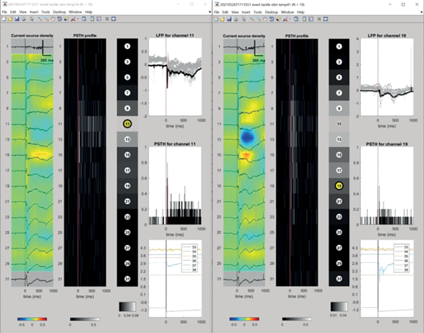
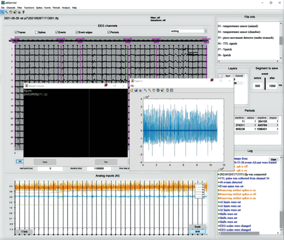
Fig. 5.
WEEGIT interface view 5, console mode is launched. An example of first time derivative for the 11th channel is presented (was built using console commands). Рис. 5. Вид 4 интерфейса WEEGIT, консольный режим включен. Представлен пример первой производной для 11-го канала (создан с помощью консольных команд).
An interactive plugin for monitoring average properties is used for estimating activity properties around the detected events. It includes a separate interactive figure, where the user is able to parse through the channels using “up” and “down” keyboard keys. On the figure the following panels are presented (from the left to right): average CSD profile of the event, Peri-event time histogram (PETH) depth profile, average spike rate depth profile, target channel average LFP (top), target channel peri-event time histogram (middle) and Analog input channels average trace (bottom).
The console tool allows the user to run and save custom code in Matlab language. Console is represented in beta-version, however, will be improved in the future release.
4. FUTURE DIRECTIONS
“WEEGIT” demonstrates a well organized environment and concept of data workflow. However, despite obvious benefits, presented software has some restrictions and deficiencies. Therefore, future release of the “WEEGIT” will cover the following key improvements: 1) Resolving filtering collapse due to the adaptive resampling rate; 2) Graphical representation of spike clusters for each channel; 3) Basic descriptive analysis for full record electrophysiological properties; 4) Events detection using spikes density raise; 5) User-friendly interface for custom analysis implementation; 6) Event viewer interactive plugin for browsing events and 7) Include reading of the *.HDF5 files as the popular format of large, complex and heterogeneous data store.
5. DISCUSSION
“WEEGIT” is able to work with wide range of the file formats of electrophysiological activity registration – *.abf, *.daq, *.csc, *.xdat, *.rhd, *.edf, *.continious. Presented formats are characterized by absolutely different internal configuration of headers and data organization, however, almost all of them store data as a raw binary data. To avoid additional workload during usage of the “WEEGIT” we decided to convert data formats to one simply organized raw binary file with header externally stored in a separate *.json file. Data from a raw binary file can be directly read with a low-level function, requiring the shortest possible time for this operation. External file for header was used, firstly, to avoid difficulties with binary file header reorganization and, secondly, for easier reading of the header with text editors. This approach also allows us to standardized data for future analysis. However, additional operation for data convert required some time and space on the hard drive, that can be a disadvantage for the users. Mechanisms of fast visualization are based on two components: 1) direct reading of the binary file and 2) adaptive sample rate of uploaded data. Usage of low-level function to read the binary file provides the fastest speed, while fixed number of time points for graphical environment reduce the required volume of random-access memory. However, that approach lead to some difficulties with filtering of the data, because of floating resampling rate. That restricts filtering in some time ranges, resulting in deficiency of this operation.
Though, we expect that WEEGIT should predominantly fit the browsing of electrophysiological recordings done with multisite linear electrode, we believe that WEEGIT will be also fruitful for pre-analysis of the electrophysiological recordings done with other types of electrodes and electrodes configurations (tetrodes, multishank, single eletrode etc) and in other systems (ECG, EMG etc). That will be associated with some functional limitations (loss of MUA or CSD analysis), however, we prepare the option to add extra scripts in “Console mode” for future releases. But, the main functions for signal filtering and transform or detection of the events can be equally used for any types of electrophysiological recordings.
The opportunity of the simultaneous fast browsing and annotation of the data in one space was highly appreciated by the ordinary users of the similar type of software. However, an overview of the popular browsers showed, that, despite obvious advantages of included analysis packages, the workflow doesn’t support a convenient way of record documenting at all. For example, in the famous software “Clampfit” (Molecular Devices) annotation capabilities are presented both with text and interactive methods. However, the record data from the file are fully placed in the Random-access memory, meaning large machine resources consumption in case of large (>10 GB) files. “Neuroscope” browser (Hazan, 2006) in opposite, provides a good engine with adaptive data upload, but on the background of poor organized annotation abilities. Modern powerful packages like Real-Time experiment Interface (Patel, 2017) or NeuroScore (CNS Software) demonstrate a complex user interface, resulted in time-consuming process of simple data browsing and annotation. Assuming that in this case more time required for the learning of all software features, those products more related to the specialists neither than to beginners. “WEEGIT” software concept is trying to keep the delicate edge between complexity of the proposed tools and user-friendly interface. Moreover, in modern research, authors prefer to use their custom-build analysis. Therefore, “WEEGIT” is designed to provide the simplest descriptive tools for the beginners with ability of immediate application of fancy analysis by console tool for professionals.
6. CONCLUSION
The “WEEGIT” software can potentially solve the problem of fast visualization and annotating of the electrophysiological activity data in the field of basic scientific research and can be applied in medicine diagnostics, for example, in description of brain EEG. The program works with the majority of widely used formats of electrophysiological activity data recording. The program does not consume significant hardware resources due to adaptive displaying algorithms. The opportunity of visualizing and documenting the observed electrophysiological activity is designed within one interface. Doesn’t require specific knowledge of programming, physiology or medicine, so it can be used with equal success by beginners and specialists in any of these fields. At the same time, the information is systematized and prepared for further analysis by more specialized algorithms. Thus, the program additionally allows optimal organization of interaction between biomedical specialized personnel and analytical department with physical and mathematical specialization.
Список литературы
Altman Y. Findjobj – find java handles of Matlab graphic objects. MATLAB Central File Exchange 2023. https://www.mathworks.com/matlabcentral/fileexchange/14317-findjobj-find-java-handles-of-matlab-graphic-objects
Buzsaki G., Anastassiou C.A., Koch C. The origin of extracellular fields andcurrents — eeg, ecog, lfp and spikes. Nature Reviews Neuroscience 2012. 13 (6): 407–420. https://doi.org/10.1038/nrn3241
Hazan L., Zugaro M., Buzsaki G. Klusters, neuroscope, ndmanager: A free software suite for neurophysiological data processing and visualization. Journal of Neuroscience Methods 2006. 155 (2): 207–216. https://doi.org/10.1016/j.jneumeth.2006.01.017
Nasiotis K., Cousineau M., Tadel F., Peyrache A., Leahy R.M., Pack C.C., Baillet S. Integrated open-source software for multiscale electrophysiology. Scientific Data 2019. 6 (1): 231. https://doi.org/10.1038/s41597-019-0242-z
Patel Y.A., George A., Dorval A.D., White J.A., Christini D.J., Butera R.J. Hard real-time closed-loop electrophysiology with the real-time experiment interface (rtxi). PLOS Computational Biology 2017. 13 (5): e1005430. https://doi.org/10.1371/journal.pcbi.1005430
Siegle J.H., Lopez A.C., Patel Y.A., Abramov K., Ohayon S., Voigts J. Openephys: an open-source, plugin-based platform for multichannel electrophysiology. Journal of Neural Engineering 2017. 14 (4): 045003. https://doi.org/10.1088/1741-2552/aa5eea
Tadel F., Baillet S., Mosher J.C., Pantazis D., Leahy R.M. Brainstorm: A userfriendly application for meg/eeg analysis. Computational Intelligence and Neuroscience 2011. https://doi.org/10.1155/2011/879716
Дополнительные материалы отсутствуют.
Инструменты
Журнал высшей нервной деятельности им. И.П. Павлова